Three classical methods of trajectory planning in the configuration space have been implemented. The first one allows the user to generate a trajectory described by cubic polynomials
[Q,V,A,T,c] = trj_poly3(T, Q0, Qt, V0, Vt)
where: T - vector containing a set of time instants for which trajectory will be generated; Q0, Qt - initial and final configuration of the manipulator; V0, Vt optional the initial and final velocity; Q - trajectory for each time instant and each joint; V, A - the instantaneous velocities and accelerations; c - matrix containing polynomials' coefficients describing the calculated trajectory.
If it is important to determine acceleration at the beginning and at the end of the motion 5-th order polynomials can be used:
[Q,V,A,T,c] = trj_poly5(T, Q0, Qt, A0, At, V0, Vt)
where: A0, At - initial and final acceleration; other parameters have a similar meaning as trj_poly3 parameters.
The third trajectory planning method implemented in the toolbox gives a trajectory described by a linear segment with parabolic blends:
[Q,V,A,T,c] = trj_line(T, Q0, Qt, A0, At, V0, Vt)
where all parameters have a similar meaning as those presented above.
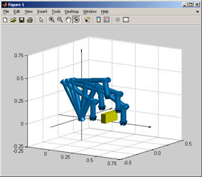
Manipulator of three mutually perpendicular prismatic joints will perform the task of movement from initial [-2.04; 2.51; 1.10] to final [-1.17; 1.7; 1.04] through its intermediate configuration [-1.79; 1.63; 1.54] (manipulator avoids the obstacle).
% workspace
axis([-0.25 0.75 -0.5 0.5 -0.25 0.75])
csys_plot(csys(eye(4), 'CSysAxisLength', axis, 'CSysAxisLabel', {'','',''}));
grid on
campos([3 -8 1.5]);
camlight
% manipulator
r = robot( [dh(0,0,0,-2.04); dh(0,0.4,0,2.51); dh(0,0.36,0,1.1)], ['r', 'r', 'r'], 'RobotBase', rp2t(rotx(-pi/2),[0;0;0]), 'RobotGrasper', [0.15; 0; -0.025], 'RobotGrasperSize', 0.05, 'RobotColor', [0,0.5,0.8], 'RobotExColor', 'g', 'RobotCylinderRadius', 0.025, 'RobotCylinderApprox', 64, 'RobotModel', 'config');
r = robot_plot(r, 'surf');
% obstacle
b = block_move(cuboid(0.05,0.2,0.1,'BlockColor','y'),[0.3;0;0]);
b = block_plot(b, 'surf');
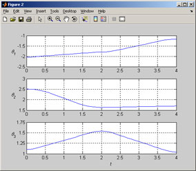
% trajectory planning
t1 = 0:0.1:2; % time definition for first section (from initial to intermediate configuration)
t2 = 2:0.1:4; % time definition for second section (from intermediate to final configuration)
% calculation of linear trajectory with parabolic blends for both sections
q1 = trj_line(t1, [-2.04;2.51;1.10], [-1.79;1.63;1.54], 1, 1);
q2 = trj_line(t2, [-1.79;1.63;1.54], [-1.17; 1.7; 1.04], 1, 1);
% motion simulation
r = robot_motion(r, [q1 q2], 0.1);
|
|
| Fig. 1. Motion of the manipulator | Fig. 2. Trajectories for individual joints |